Bloom filters: the niche trick behind a 16× faster API

This post is a deep dive into how we improved the P95 latency of an API endpoint from 5s to 0.3s using a niche little computer science trick called a bloom filter.

We’ll cover why the endpoint was slow, the options we considered to make it fast and how we decided between them, and how it all works under the hood.

Intro

A core concept of our On-call product is Alerts. An alert is a message we receive from a customer’s monitoring systems (think Alertmanager, Datadog, etc.), telling us that something about their product might be misbehaving. Our job is figure out who we should page to investigate the issue.

We store every alert we receive in a big ol’ database table. As a customer, having a complete history of every alert you’ve ever sent us is useful for spotting trends, debugging complex incidents, and understanding system health. It’s also helping us build the next generation of AI SRE tooling.

We surface alert history in the dashboard. Here’s an example of ours today:

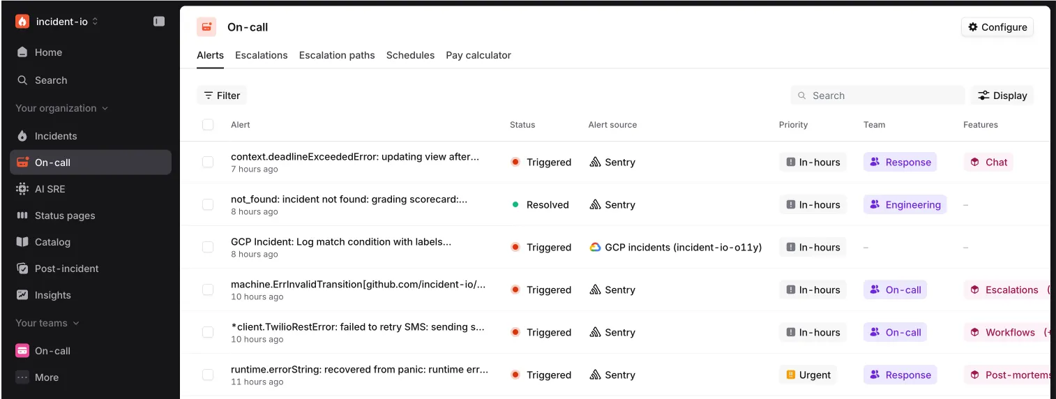
This is cool, but for large organisations with lots of alerts, this view isn’t very helpful. They want to be able to dig in to a subset of this data. The little “Filter” button in the UI lets you do exactly that.

You can filter by things like source and priority. Source is the monitoring system that sent the alert, and priority is configured on a per-customer basis and provided in the alert message we receive.

In our set up, we have these “Team” and “Features” columns in the UI too. Teams are a first class citizen in incident.io, but a “Feature” is a concept that we’ve defined ourselves. Both are powered by Catalog. Any incident.io customer can model anything they want in Catalog, and then define rules to tell us how to match an Alert to a specific entry.

This is now really powerful. For example, I can ask for “alerts with a priority of urgent or critical, assigned to the On-call team, affecting the alerts feature”:

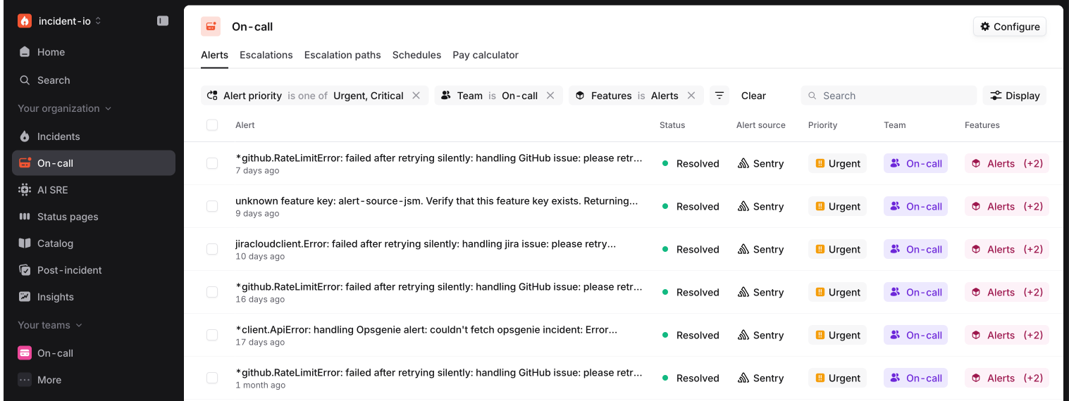
These filters are great for our customers, and, as we found out, a potential performance nightmare for us. As we’ve onboarded larger customers with millions of alerts, our slick, powerful filtering started to feel… less slick.

Some customers reported waiting 12 seconds for results. Our metrics observed the P95 response time for large organisations at 5s. Every time they loaded this page, updated a filter, or used the infinite scrolling to fetch another page, they looked at a loading spinner for far too long.

How filtering works (and why it was slow)

Let’s start with how we store alerts in our Postgres database, and the algorithm we use to fetch a filtered result set.

Here’s a simplified representation of our alerts table:

  +----------+------------------+----------------------+------------------+--------------------------------------------------+
  | id       | organisation_id  | created_at           | priority_id      | attribute_values                                 |
  +----------+------------------+----------------------+------------------+--------------------------------------------------+
  | $ALERT1  | $ORG1            | 2025-10-31 00:00:00  | $lowPriorityID   | {                                                |
  |          |                  |                      |                  |   "$myTeamAttributeID": "$onCallTeamID",         |
  |          |                  |                      |                  |   "$myFeatureAttributeID": "$alertFeatureID"     |
  |          |                  |                      |                  | }                                                |
  +----------+------------------+----------------------+------------------+--------------------------------------------------+
  | $ALERT2  | $ORG2            | 2025-10-31 00:01:00  | $highPriorityID  | {                                                |
  |          |                  |                      |                  |   "$myTeamAttributeID": "$responseTeamID"        |
  |          |                  |                      |                  | }                                                |
  +----------+------------------+----------------------+------------------+--------------------------------------------------+

id is a ULID: a unique identifier that’s also lexicographically sortable. We use them to implement pagination. $ALERT{N} isn’t a valid ULID, but it is easy to read in a blog post.
organisation_id is another ULID, identifying the organisation/customer.
created_at is a timestamp that does what it says on the tin.
priority_id is a foreign key that references your organisation-specific priorities. Each incident.io customer can define the priorities that work for them.

When you set up an alert source like Alertmanager, you specify the “attributes” we should expect to find in the metadata we receive - in this example: priority, team and feature. First-class dimensions like priority have their own columns in the database, but everything else that’s custom to you is stored as attribute_values in JSONB.

Extracting attributes from alert payloads

The algorithm to compute a filtered result set works like this:

Construct a SQL query including filters that can be applied in-database
Fetch rows from the database in batches of 500, and apply in-memory filters
Continue fetching batches until we’ve found enough matching alerts to fill a page

Let’s work that through using the same example as above. The infinite scrolling UI hides pagination parameters, but they’re always defined behind the scenes. Let’s ask for “50 alerts with a priority of urgent or critical, assigned to the On-call team, affecting the alerts feature”.

Priority has its own column in the DB, so we can get Postgres to do that filtering for us. The SQL to get the first batch of alerts looks something like:

SELECT * FROM alerts WHERE
  organisation_id = '$ORG1'
  -- the priority filter can be applied in the DB
  AND priority_id IN ('$highPriorityID', '$criticalPriorityID') 
-- pagination (more on this in a mo)
ORDER BY id DESC
-- batching
LIMIT 500

We fetch 500 rows from the DB into memory. Our ORM deserialises the rows into Go structs. Now we need to apply the attribute filters, which means deserialising the JSONB into more Go structs. We check the team and feature attributes of each of the alerts in the batch, and we find 10 that match. We’re trying to fill a page of 50, so we have to make another SQL query for a second batch:

SELECT * FROM alerts WHERE
  organisation_id = '$ORG1'
  -- the priority filter can be applied in the DB
  AND priority_id IN ('$highPriorityID', '$criticalPriorityID')
   -- if we have 5000 alerts, this skips the first 500 alerts
  AND id < '$ALERT4500'
ORDER BY id DESC
LIMIT 500

We keep doing this until we’ve found 50 matching alerts.

We have a B-tree index on (organisation_id ASC, id DESC) called idx_alerts_pagination designed for this exact use case, which theoretically makes the query for each batch nice and efficient.

However, the worst-case scenario for this algorithm is when the in-database filters don’t exclude many rows, forcing us to fetch many batches to apply in-memory filters to. A key bottle neck here is deserializing the row and JSONB data into their respective structs. Our telemetry showed us that fetching and deserializing a batch of 500 rows from the DB took ~500ms, with only ~50ms of that spent waiting for the query to return results.

You might also be thinking, “why do the attribute filtering in memory?”. Good question. I mentioned in the intro that alert attributes are backed by the Catalog. The Catalog is really powerful, and I’ve used a simplified illustration of what we store in the JSONB to try and stay on topic. In reality, attribute values can be scalar literals, arrays of literals, references to other Catalog entries (like a Team), or even dynamic expressions (e.g., "assignee is the CTO if P1, else the owning team"). It’s complicated, and I’d like to get on to the bloom filtering bit, so please just trust me that it was a reasonable design decision at the time!

How to go faster

Our bottleneck is fetching and deserializing large amounts of the data from Postgres. Therefore our best bet to go faster is to push as much filtering in to the DB as possible, This means we need Postgres to be able to efficiently use the attribute_values data to filter alerts.

We spiked two options.

Option 1: A GIN Index. This is the "standard" Postgres answer. GIN (Generalized Inverted Index) is designed for indexing complex types, including jsonb. We could create an index on the attribute_values column and use the jsonb_path_ops operator.

Option 2: Bloom filters. This was an idea proposed by Lawrence Jones, one of our founding engineers. By encoding our attributes values as bit strings, Postgres could rapidly perform bitwise “one of” operations for us.

What the hell is a bloom filter?

Indeed.

A bloom filter represents a set of items. We can check the existence of an item in the set and get one of two answers:

The item is definitely NOT in the set
The item MIGHT be in the set

In exchange for the probabilistic nature of the filter, we can perform very efficient queries in terms of time and space.

The set itself is a binary representation of all of the items called a bitmap.

Items are added to the set by computing multiple hashes that each return a value corresponding to an index in the bitmap.

To check if an item exists, we use the same hashing functions on the item to produce another binary representation called a bitmask.

Using the bitmap and bitmask we can use bitwise logic to very efficiently run the check:

bitmap & bitmask == bitmask

Let’s walk this through with a contrived example:

Bitmap: 8 bits (positions 0-7), initially all 0s
Hash functions: h1, h2, h3 (each returns 0-7)

To add an item to the set, we apply the three hashing functions, each of which returns a value corresponding to an position in the bitmap. We set the bitmap values at each of these positions to 1. To add multiple items, we repeat the process:

Add "apple":
  
        "apple"
       ┌───┼──────────┐
       ↓        ↓     ↓
      h1       h2    h3
       │        │     │
       2        5     7
       ↓        ↓     ↓
[0][0][1][0][0][1][0][1]
 0  1  2  3  4  5  6  7

Add "banana":
  
        "banana" 
    ┌──────┼────┐
    ↓     ↓     ↓
   h1    h2    h3
    │     │     │
    1     3     5
    ↓     ↓     ↓
[0][1][1][1][0][1][0][1]
 0  1  2  3  4  5  6  7

To check if an item is in the set, we use the same three hashing functions to compute another three bitmap positions. If ALL of those positions in the bitmap are 1, the item MIGHT be in the set. If ANY of them are 0, the item is definitely NOT in the set. This is the logical AND operation:

Check "apple":
  
        "apple"
       ┌───┼──────────┐
       ↓        ↓     ↓
      h1       h2    h3
       │        │     │
       2        5     7
       ✓        ✓     ✓  = ✅ MIGHT be in set
[0][0][1][0][0][1][0][1]
 0  1  2  3  4  5  6  7

Check "cherry":
  
        "cherry"
    ┌──────┼───────┐
    ↓        ↓     ↓
   h1       h2    h3
    │        │     │
    1        4     6
    ✓        ✗     ✗    = ❌ NOT in set
[0][1][1][1][0][1][0][1]
 0  1  2  3  4  5  6  7
      
      
Check "grape":
  
        "grape"
    ┌──────┼────┐
    ↓     ↓     ↓
   h1    h2    h3
    │     │     │
    1     3     5
    ✓     ✓     ✓       = ⚠️ MIGHT be in set
[0][1][1][1][0][1][0][1]  (false positive!)
 0  1  2  3  4  5  6  7

The size of the bitmap and number of hashing functions can be tuned to trade off storage space and false positive rates. We can reduce the false positive rate by increasing the size of the bitmap, and then using more hashing functions so that each item is represented by more bits.

The bottleneck in our alert filtering algorithm is fetching and deserializing large amounts of the data from Postgres. Therefore our best bet to go faster is to push as much filtering in to the DB as possible. How do bloom filters help us do that?

Firstly, we need to be able to treat attribute value filters as set operations.

If an alert has the following JSONB attribute values:

{
  "$teamAttributeID": "$onCallTeamID",
  "$featureAttributeID": [
    "$alertsFeatureID",
    "$escalationsFeatureID"
  ]
}

using a simple encoding to represent an attribute value as a string, we can represent these attributes values as a set of strings:

{
  "$teamAttributeID:$onCallTeamID",
  "$featureAttributeID:$alertsFeatureID",
  "$featureAttributeID:$escalationsFeatureID"
}

Now a search for alerts with a given attribute value is a set operation - we check to see if the string encoded ID and value we’re searching for are present in this set.

We can turn our set of attribute values into a bloom filter by hashing each string-encoded item to compute a bitmap. We can also represent an attribute value we want to filter by as a bitmask, and use bitwise logic to get our efficient-but-probabilistic answer.

There’s some neat maths to figure out how many bits you need in your bitmap, and how many hashing functions you need to apply in order to achieve a target false positive rate for a given cardinality. For us to achieve a 1% false positive rate across all attribute values in the alerts table, we needed 512 bits and seven hashing functions.

Computing the bitmap looks the same as the toy example above, just with more hashing functions and more bits:

Add "$teamAttributeID:$onCallTeamID":

            "$teamAttributeID:$onCallTeamID"
         ┌─────┬─────┬─────┼─────┬─────┬─────┐
         ↓     ↓     ↓     ↓     ↓     ↓     ↓
        h1    h2    h3    h4    h5    h6    h7
         │     │     │     │     │     │     │
         2    17    143   216   342   487   501
         ↓     ↓     ↓     ↓     ↓     ↓     ↓
[0] [0] [1]...[1]...[1]...[1]...[1]...[1]...[1]...[0] [0]
 0   1   2    17    143   216   342   487   501   510 511

We compute this bitmap every time an alert’s attribute values change. We store it in attribute_values_bitmap column in Postgres, as a Bit String Type: bit(512).

When we want to find alerts matching some attribute filters, we compute bitmasks using the same key-value pair string encoding and hashing functions. Postgres can do the bitmap & bitmask == bitmask for us, and rapidly, thanks to the Bit String Type.

Here’s the SQL query for “50 alerts with a priority of urgent or critical, assigned to the On-call team, affecting the alerts feature”:

SELECT * FROM alerts WHERE
	organisation_id = '$ORG1'
	-- the priority filter can be applied in the DB
	AND priority_id IN ('$highPriorityID', '$criticalPriorityID') 
    -- we can now also filter attribute values in the DB!
	AND attribute_values_bitmap &amp; '$onCallTeamBitmask' == '$onCallTeamBitmask'
	AND attribute_values_bitmap &amp; '$alertsFeatureBitmask' == '$alertsFeatureBitmask'
ORDER BY id DESC -- pagination
LIMIT 500 -- batching

Our 1% false positive rate means we now have 1% of the deserialization work to do than we did before. We do still have to check the results we get back in memory, to remove false positives, but that’s now very manageable overhead.

Neat!

GIN vs bloom

Now we know how bloom filters work, let’s get to our spike results.

We prototyped each option, and measured the performance of a couple of key scenarios to evaluate them. Here’s the results:

	GIN	Bloom
Scenario 1: Frequent alerts	150ms	3ms
Scenario 2: Infrequent alerts	20ms	2-300ms

Both scenarios are based on an organisation with ~1M alerts. “Frequent alerts” refers to a query that matches ~500K of the 1M alerts, and “infrequent alerts” to a query that only matches ~500.

The GIN index query plan looked like:

Use the GIN index to efficiently find all the alerts that match the filters
Read all of the alerts
Sort and take the top 500

This is really fast when 500 alerts match the filters. When 500K alerts match the filters, we have to read all 500K to sort them, only to throw away 495.5K for our LIMIT 500 clause.

The bloom filter’s query plan looked like:

Use idx_alerts_pagination to “stream” alert tuples sorted by ID
Filter the “stream” using efficient bitwise logic
Continue until 500 matching tuples are found

This is really fast when 500K alerts match the filters, because we have a 50% chance that any one alert matches, so we end up reading only a small part of the index. When 500 alerts match, we have a 0.05% chance that each alert matches, and we end up reading much more of the index.

The latencies are well within bounds for a much improved user experience, and we couldn’t think of a good reason why one of the frequent or infrequent alert scenarios was preferable to the other, so we called this a draw from a performance perspective. However, we’d illustrated a critical issue with both options - they scale with the number of organisation alerts. We keep a complete history of customers’ alerts, so whilst either would deliver what we wanted now, performance would degrade over time.

Time makes fools of us all

Whilst drunk on maths and computer science, something really simple had been staring us in the face.

We use pagination to sort alerts by the time we receive them, and we show customers their most recent alerts first in the UI. Most of the time they’re interested in recent history, and yet our queries can get expensive because we’re searching all the way back to the first alert the ever sent us. Why? If we can partition our data by time, we can use this very legitimate recency bias to realise a lot of performance.

The available filters in the dashboard include one for the created_at column we have in the alerts table. We made this mandatory, and set 30 days as a default value. We even had an idx_alerts_created_at index on (organisation_id, created_at) ready to go!

The GIN index query plan now uses two indexes:

Intersect indexes to find all recent alerts that match the filters
1. idx_alerts_attribute_values applies the filters
2. idx_alerts_created_at finds alerts in the last 30 days
Read all of the alerts
Sort and take the top 500

The bloom filter query plan doesn’t need to change at all, thanks to a very useful detail we touched on at the start. Our alert IDs are ULIDs - unique IDs that are lexicographically sortable. ULIDs have two components; a timestamp and some “randomness”. We can use “30 days ago” as a timestamp, stick some randomness on the end, and use it in a range query with idx_alerts_pagination.

Both query plans still technically scale with the number of organisation alerts, but the amortized cost is now much better. Customers can select large time ranges to analyze, which might take some time to process, but we’re trading that off against the performance we gain for much more common use cases. We’re going to have to onboard customers with biblical alert volumes before the default 30 day window will cause UX issues. That’ll be a nice problem to have, and one we don’t feel the need to design for now.

Now we’ve solved the scaling issue, we’re back at our stalemate. How to pick one to implement?

The debate that followed was what you might call “robust”. Respectful, but rigorous.

GIN indexes can be large, on disk and in memory, and have high write overhead. We were concerned that as the index bloated, it could take up too much space in Postgres's shared buffers, potentially harming performance in other parts of the platform. We didn't have high confidence that we wouldn't be back in a few months trying to fix a new, more subtle problem.

Bloom filters are a pretty niche topic, we thought the code would be hard to understand and change if you weren’t involved in the original project, and we felt uncomfortable about essentially implementing our own indexing mechanism - that’s what databases are for.

In the end we were very resistant to the idea of re-work. We bet on the thing we were confident we’d only have to build once, even if it was a bit more complex - the bloom filter.

Conclusion

Combining the mandatory 30-day time bound with the bloom filtering has had a massive impact: the P95 response time for large organisations has improved from 5s to 0.3s. That’s a ~16x improvement! The bloom filter reduces the number of rows in each batch, and the mandatory time bound reduces the maximum number of batches.

Our powerful and slick filtering is slick again, and it should stay slick as we continue to onboard large customers. As of September 2025 we ingest more than a million alerts per week, and that number will only increase!

This is a great example of how technical and product thinking can go hand in hand. However you go about it, this is one of those hard technical problems to solve, and I’m lucky to work alongside incredibly talented engineers. However, understanding our customers and how they use our product led us to a vital piece of the puzzle. We needed both to really nail this.